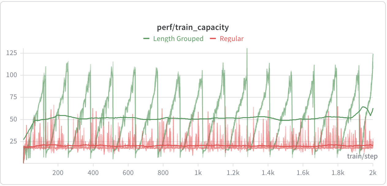
Over the last few weeks, we have been working on increasing the training speed of speculative decoding to get maximum performance. Speeding up training would make speculative decoding research and experimentation more accessible. In summary,
We believe our changes will democratize speculative decoding research and experimentation while making it easier to get started and faster to run.
Speculative decoding training can be sped up in two ways: increasing number of data-parallel workers and increasing batch size. The latter works well since training is largely memory bandwidth bounded due to EAGLE TTT calculations. However, a naive scaling doesn't scale linearly. If we look deeper, we see this is caused by excessive padding added to the input sequences to match the sequence dimensions of the model across different GPUs and batches.
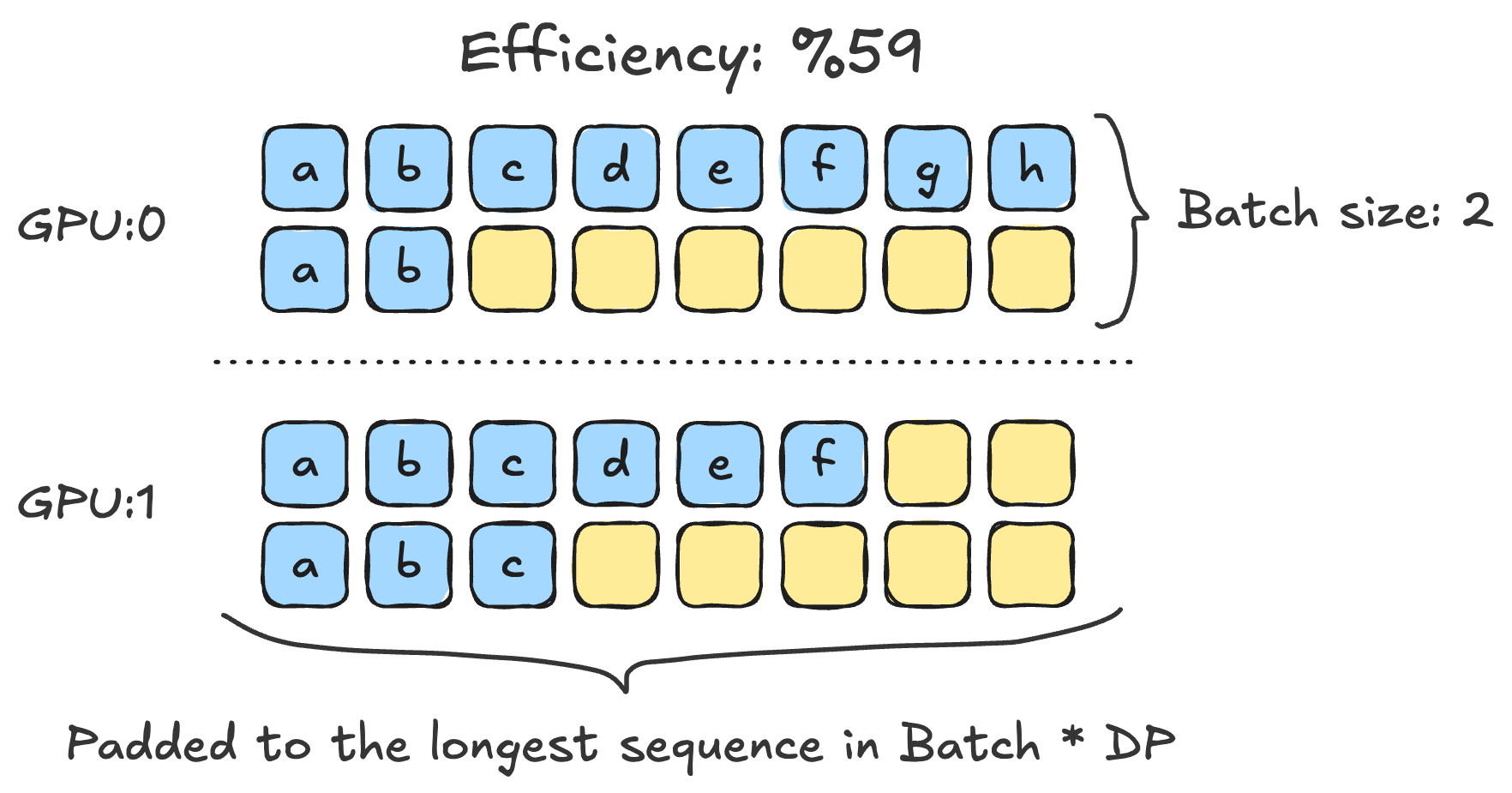
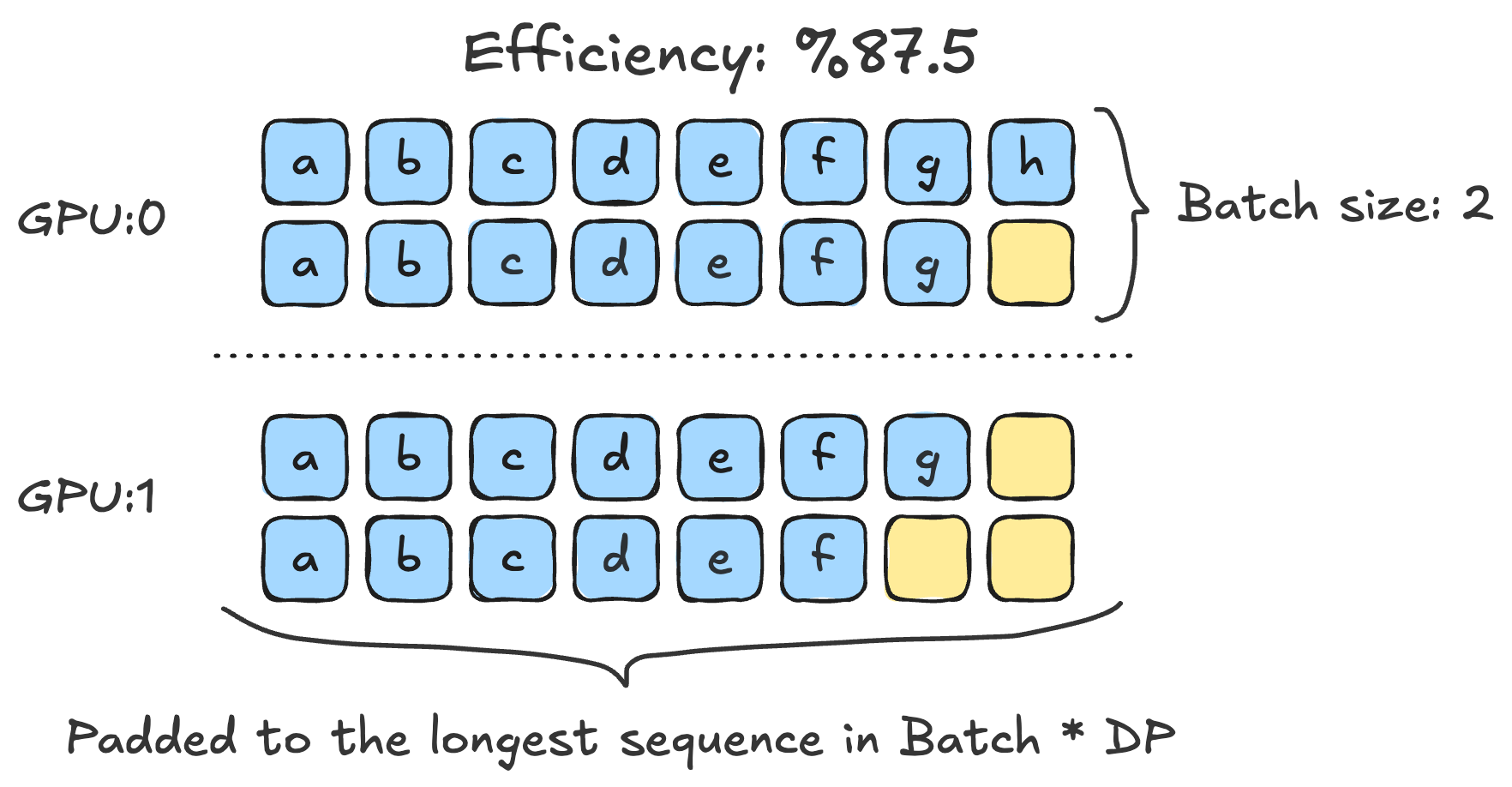
To address this, we have sorted the sequences by length and grouped them into batches of similar lengths. This minimizes padding and improves training speed.
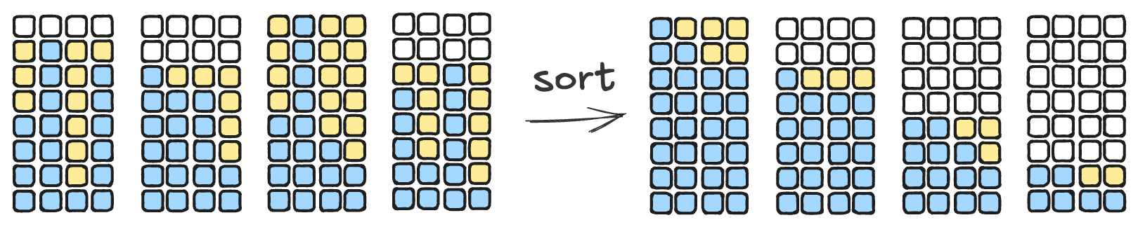
After grouping, the efficiency is improved, the yellow squares are excess padding, white squares are padding that we can omit.
Eliminating CPU .item() and metric deferral
Another cause of slowdown was the use of .item() in the main thread. Those calls were making the main thread wait until GPU operations were completed. However, some of them was not avoidable, such as metrics. So we've deferred the metric reporting by 1 step, the main thread does not need to wait for GPU operations for the current operation. Moreover, we have switched to the fused Adam optimizer and replaced our for loops with torch._foreach_ loops to speed up training.
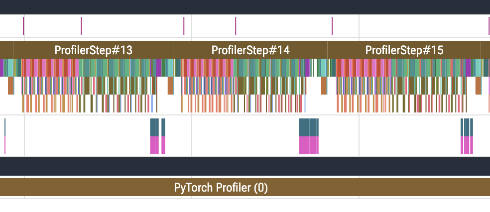
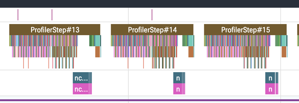
We made our tokenization and data processing step 4.5x faster.
Some context on what this step does. Before training starts, we convert a million raw conversations into token IDs. This happens once and the result is cached, but it sat on the critical path for every fresh dataset, and it was slow enough to be painful. The work is split across two stages. A single parent process reads the conversations and cleans them up, then hands them to a pool of 64 worker processes that do the actual tokenizing.
Finding 1: the workers were sending results back in an expensive format.
Collecting 1M rows of results from the workers took 498 seconds and after the fix it takes 23 seconds.
Each worker tokenizes a conversation and sends the result back to the parent. We were sending PyTorch tensors. When PyTorch sends a tensor between processes, it does not copy the data through the pipe. Instead it places the data in shared memory and passes a handle to it, so the receiving process can read the same memory directly. This is usually the fast path, and for a handful of large tensors it is.
The problem is that every tensor gets its own shared memory segment, and every segment costs one file descriptor. File descriptors are a limited per-process resource. With a million samples, the parent process runs out of them.
NumPy arrays have no such mechanism. They get sent as plain bytes, and the parent turns them back into tensors with torch.from_numpy, which reuses the same memory rather than copying it. So the workers now return NumPy and the parent converts. Less clever, much faster.
Finding 2: the workers were inheriting a copy of the entire dataset they never needed.
Tokenizing 1M rows took 1436 seconds, after the fix it takes 319 seconds.
The worker pool was being created after the parent had finished reading all one million conversations into memory. On Linux, starting a worker process is cheap because the child does not copy the parent's memory. It shares it, and only makes a private copy of a page when it writes to that page. This is called copy-on-write, and it usually means an idle inherited object costs nothing.
However, every Python object carries a reference count in its header, and that count changes whenever the object is touched, even just to read it. So a worker that merely looks at inherited data writes to it, which forces a private copy of the page. Multiply by 64 workers and roughly 22.8 GB of conversations each, and the machine starts copying more than a terabyte of memory for no reason.
The fix is to create the pool before the parent loads anything. The workers then inherit an empty list instead of a full corpus, and they receive their actual input through the normal work queue, which is what they were always reading from anyway.
Normally TorchSpec runs the target model and the draft trainer at the same time, on the same box. The target model generates hidden states, ships them through Mooncake, and the trainer consumes them. That works, but it means you need multiple GPUs and you should carefully load balance, whichever side is slower throttles the other. Therefore in some cases users might prefer to run offline training, for example if they have a lot of disk space or if they are constrained on GPUs and doing experimentation on a small dataset.
Offline training splits this into two phases. First you run the target model once and write every hidden state to disk. Then you train against those files, with no target model running at all.
# Phase 1: materialize hidden states (uses the inference GPUs)
python -m torchspec.offline.generate \
    --config configs/your_config.yaml \
    --output ./data/hidden-states

# Phase 2: train against them (all GPUs free for training)
# in your config:
#   inference:
#     inference_engine_type: offline
#     offline:
#       data_path: ./data/hidden-states
# num_engines: 4Each sample stores the target model's auxiliary hidden states, its final hidden state, and the input token IDs:
where $L$ is the sequence length in tokens, $H$ the target model's hidden size, $A$ the number of auxiliary layers EAGLE-3 captures, and $b$ the bytes per element.
| dataset | $\bar{L}$ | predicted | measured |
|---|---|---|---|
| 16k rows, cap 8192 | ~3,240 | 1.7 TB | 1.7 TB |